
google sheet vlookup 多條件
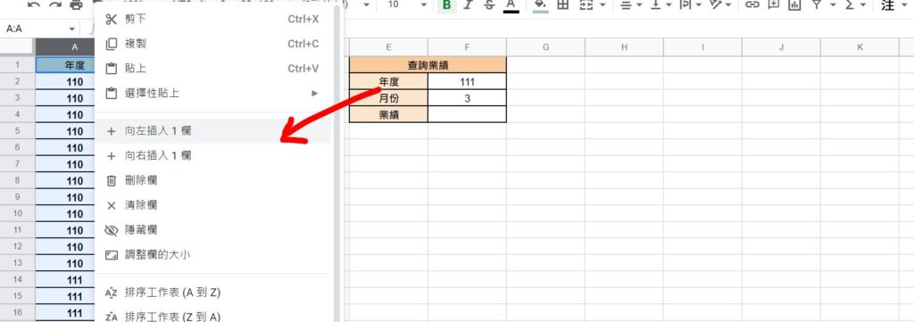
Step 1 在A欄位點擊滑鼠「右鍵」,並選擇「向左插入1欄」

Step 2 輸入公式「=B2&C2」,將要查找的兩個條件儲存格合併起來,並向下填滿
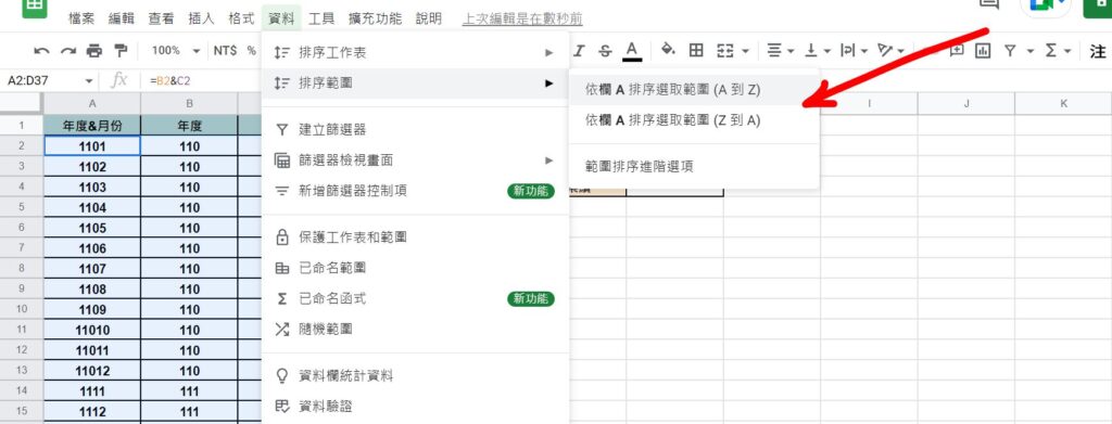
Step 3 將儲存格範圍選取,在上方功能列「資料」中「排序範圍」選擇「依欄A排序選取範圍(A到Z)」
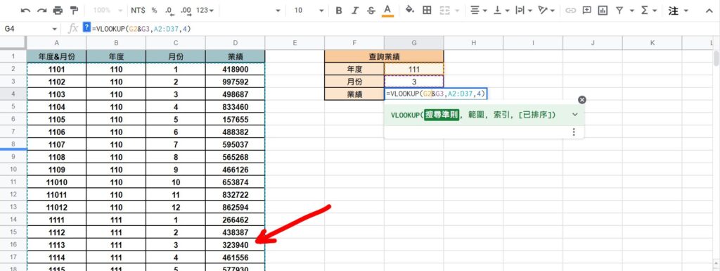
Step 4 使用VLOOKUP函數,輸入公式「=VLOOKUP(搜尋準則,範圍,索引,[以排序])」,將範例代入公式「=VLOOKUP(G2&G3,A2:D37,4)」,即可達成多條件查找資料表